
A bit of statistics, but just a little
Let us now see the meaning of the two terms that distinguish the two methods. I will do it without going into specific statistical terms, and I do not want the purists of the subject, but my aim is to have already made calculations used, to make life easier for the trader who must understand simply how to read the indicator that is proposed. Moreover, not having invented the demonstration of the phenomenon, it will be sufficient to read the formulas of Engle Granger that are those used for the calculations.
I begin by re-proposing the classic. An example that is quoted to help in understanding the different meaning of two terms that apparently indicate an equal property.
Correlation
Imagine watching two drunks coming out of a bar heading home and suppose that, although they both live in the same neighborhood, they do not know each other or decide to tackle different paths to return to their homes. They will therefore have a relationship that unites them and therefore we could at all times measure it by calculating the distance that separates them from their destination. Since the goal is coincident for both, at each measurement interval we can construct their correlation level. At 5 minute intervals they approach the goal, not necessarily with linearity. But they come closer and therefore are related.
By correlation statistics we mean a relationship between two random variables such that each value of the first variable corresponds with a certain regularity to a value of the second in a time interval ‘t’. Please note that it is not necessarily a question of measuring a cause-effect relationship, but simply of the tendency of one variable to vary in function of another.
Cointegration
Imagine now watching a drunk who walks the dog. This time there is a relationship between the path followed by the master and the one followed by the dog, but what is the nature of this relationship? Despite the paths of the dog and that of his master are
fundamentally random (random-walk) and unpredictable, given the position of one of the two, we can however get an idea of where the other can be found. This is because the distance that separates them, although variable during their random journeys, is however limited by the length of the leash. In this case the two paths are defined as cointegrated, and this regardless of the respective correlation levels measurable in specific time intervals.
In statistics the cointegration test looks for the existence of a ‘stable’ relationship existing between two or more time series with stochastic or apparently random trends.
The cointegration test calculates in practice the value of a coefficient (sigma) δ (called the cointegration coefficient) such that the difference
Yt−δXt
that is, that the position of the dog Y, minus the position of the man X multiplied by this sigma coefficient measured at the same instant ‘t’, is a stationary time series.
What does it mean? It means that graphically you will see a sort of cyclic track (a sinusoid), formed by values whose average is equal to zero, and whose distance with respect to the average in an entire cycle is constant. Practically I will expect a return to the average when this line is at the maximum distance of its course.
Advantages By using the cointegration analysis with respect to correlation, greater stability is ensured over time, increasing the probability of profit in mean-reverting strategies, ie returning to the average.
That means that after having found the couple, we will seek the maximum divergence between the two titles that compose it, knowing that for the properties returning to the average, they will make their distance converge. It is clear that if we sold the stock which will return to the value of its average (lower) and bought what will instead return to the value of its average (higher), we would have our profit.
Note: not the opposite because, starting from when they are converging, we would not know which way they will diverge.
The principle, I repeat, is the return to the average, NOT the departure from the average.
In practice we will make the measurement of the OverSpread graph and when it will distance itself from its average reaching the maximum probable values we will enter position expecting the return to the average, that is to the position 0.
How do we define which are the maximum values?
There is a measurement that if done on the difference in the average price allows us to define the maximum and minimum values. This measurement is called standard deviation. The standard deviation is calculated in 4 steps.
The first is to calculate the average of the Close.
The second step consists in calculating how much each Close differs from the Close of an average of 10 bars, and since the value could be negative, these differences are squared.
The third step consists in calculating the sum of all the results obtained in the second step, and dividing them by the number of bars, that is in our case 10. The result we get is called variance.
The fourth and final step is to calculate the square root of the variance, finally obtaining the value called standard deviation.
The standard deviation is a numerical representation of how much the Close of that sample deviate from their mean. If our measurement had been made on the prices of an Italian title, the standard deviation would be expressed in euros.
An example will make everything clearer.
The Close reported in the 10 days are: 8, 6, 7, 7, 9, 6, 7, 9, 4, 7.
(8 + 6 + 7 + 7 + 9 + 6 + 7 + 9 + 4 + 7) / 10 = 7
(8 – 7) 2, (6 – 7) 2, (7 – 7) 2, … , (4 – 7) 2, (7 – 7) 2
1 + 1 + 0 +… 9 + 0/10 = 20/10 = 2
Square root of 2 = 1.41
The Close standard deviation, calculated over the 10 periods, is € 1.41.
Therefore, considering all the assumptions related to the Gaussian distribution of the Close, we can state that the value following these 10 Close, will have a 98% probability of being between the average of the Close + 2 times 1.41 and the same average – 2 times 1.41, ie it will have 98% of remaining inside 9.82 and 4.18.
The Gaussian distribution (Bell Curve) is represented in the following image:
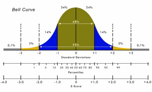
To simplify the measurements and their interpretations we used a small trick, the Z-Score.
Z-score is a statistical measure that represents the relationship between a value and the average of the values of a group to which it belongs. A value of Z-score = 0 means that the score is equal to the average. It can take positive values and negative values indicating if it is above or below the average and how many standard deviations.
If we wanted to calculate it on the Close prices, the formula would be: Close – average of Close / standard deviation … or movement / deviation.
In this way we have a value that is comparable between titles of different prices.
The OverSpread is a graph, expressed in Z-Score, centered on zero and whose scale is coincident with the values of the Gaussian bell. All the graphs of any pair of instruments will therefore have the same scale, and therefore will always be comparable to each other, and all will always have the same interpretation: if the graph reaches the value of +2 or -2 Z-Score, it means that I have only about 2% probability of continuing beyond these extreme values, and about 98% probability of returning to the central value.
It is clear that with these probabilities it is possible to identify excellent trading opportunities, which is difficult to obtain with the simple correlation. Indeed, the more the instruments are correlated, the less likely they are to earn. As promised at the beginning of this writing I will show you:
We take 2 perfectly correlated A and B instruments, that is to say the movement of 1 € of A corresponds to a movement of 1 € of B in the same direction, it is obvious that they will never have a divergence, and therefore I will never get any gain.
In fact the market risk is transferred to the yield differential: if the securities pair is chosen incorrectly, an almost insured loss is incurred.
The remedies and some caution techniques
So far we have read that the spread consists of using a pair of instruments. We must bear in mind that equity stocks should NOT be sold short for several reasons, the cost of stocks lending, the revocation without condition of this loan, the ex post prohibition that could be placed at that position. For this purpose it is better to use futures which allow short and long positions to be taken simply by subtracting the guarantee margin, which is that portion of money withheld by the Cassa Margine e Compensazione to guarantee the counterparty. It is therefore possible to keep the Short position until the Future expires simply by having enough money in the account for the margin.
Another way to build the OverSpread is to implement it using the Options. In this case, longer expiries than those of the Future can be used and the cost of the transaction is the same, remaining in both cases at around 25% of the cost directly using the titles.
Having then an OverSpread built with the options you can take advantage of all the strike defense techniques, such as rolling.
Another technique could be that to define the time of the first intervention and the threshold of the intervention, in practice it is defined after what adverse percentage must intervene and which options to buy to cover the future.
For example, suppose that in my couple the Long title I bought for 8 euros is going wrong.
Suppose we have decided that € 0.5 of adverse movement would have triggered my “B” plan and that the plan consisted of buying a 6.5 strike option, doing so I defined my maximum loss in that direction, being able to easily face an excursion of even 100% as the maximum loss and the resulting margin will not increase beyond the pre-set threshold of 8 – 6.5 = 1.5 euros.
Or combine Options and Future:
Now it’s about identifying the pairs and having the control console to complete the OverSpread once it has started. For this purpose we have included in beeTrader, software of our conception, the OverSpread function.